
The examples
Every new synthesiser should have some example
sounds. The first thing to understand is that I have
no pretensions to being either a sound designer or a
performer, so this page is intended to introduce a few
features rather than to impress with flashy sounds.
In the computer graphics community there is a motto that
'Reality is a measure of complexity' rather than an end in
itself. The point behind this motto is that if you
can control complexity well enough to produce a convincing
picture of a teapot, then you can also produce pictures of
imaginary objects that are detailed enough to fool the
viewer.
It's the same with sounds. If you want the sound of a
real instrument then you will use that instrument if the
music you have written is playable, and samples if
not. But if a synthesiser can create from scratch
convincing and controllable imitations of real sounds, then
it should also be able to produce interesting and
controllable new sounds.
I didn't choose this because I think I can produce the best possible organ sound, or because I think the Frequency Domain architecture is better suited to this than to other sounds. The physics of organ pipes are reasonably complex without being overwhelming, and there is an obvious set of parameters which can be used to generate a whole family of sounds from a single voice. (And for performance testing, I can quickly bring any computer to its knees just by pulling out more stops!)
The voice is based on the description of pipes given in "The physics of musical instruments" by Neville Fletcher and Thomas Rossing. It uses 37 modules, most of which are taken up with clumsily building up mathematical formulae one step at a time (something I'll probably address in the future), and publishes 9 parameters.
To save you from going cross-eyed, I shan't be showing you the internal details of the voice here, but I can show you how it appears to the performer. The screen shot shows the synthesiser's "Edit program" page. The synthesiser supports a generalisation of the idea of layered programs, with any number of layers, and any performance parameters controlling them. So we have one layer for each rank of pipes and one parameter for each stop. All the layers use the same underlying voice, which models an open flue pipe. (The voices for closed flues and cylindrical reed pipes are easily derived from this model. Conical reeds and flues with chimneys are slightly more complex.)
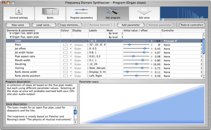
The table shows a single layer and the parameter values associated with it. A note is being played and the real-time display at top right shows the resulting spectrum.
The voice publishes a number of parameters which control the sound. These parameters may be used either as conventional real-time performance controls, or as they are here, to generate a family of related sounds. This use of parameters to generate a family of sounds invites an obvious comparison with time domain modelling synthesisers.
The difference lies in where the parameters come from. In time domain modelling the software itself embodies the model and determines the available parameters - the sound designer cannot suddenly decide to add a new parameter.
By contrast, frequency domain synthesis allows at least moderately complex models to be built by the sound designer, without assistance from a programmer, using only standard modules. All of the assumptions and simplifications that I made when I was creating this voice are visible for you to inspect, and to change if you disagree with them.
The synthesiser also allows you to mix and match different approaches. In this voice the losses and end corrections which shape the pipe resonances have been modelled (more or less carefully) using formulae from the book I mentioned above. By contrast, the air reed is modelled using a more conventional approach – one of the standard modules generates spectra which match those of standard waveforms, and I use that module here. The envelopes (controlled by the "Voicing" parameter) have the most difficult mathematics of all, so I just sketched them out by hand to match empirical measurements. In each case, you're in control and you go into just as much or as little detail as you need to get the voice how you want it.
The resulting voice offers quality comparable to that available with a fixed time domain model of an organ pipe, but the frequency domain model is much more open and flexible.
So what does it sound like? I can't play for toffee, but here goes:-
The principal stop shown above was used for the first example, the Little Prelude in D (click to play the MP3 file, or control-click to download it) from the Clavier-Büchlein BWV 925 (although it's probably not by Bach). Of course, the sound of a diapason was never intended to be used as a solo stop, so this example is probably the epitome of dullness. I include it for those who know what a diapason actually sounds like.
These examples all download as zip files to avoid a browser problem with downloading with .m4a files. If your browser does not automatically unzip downloaded files you will need to do this yourself.
The second example is the Two Part Invention in E minor BWV 778. This uses 8' and 2⅔' flute stops - a more distinctive sound and therefore a slightly easier test.
Both of these examples use John Barnes' temperament.
This is more economical, using 24 modules, two oscillator blocks (each course on the lute is made up of two strings, the lower courses tuned in octaves and the upper tuned in unison) and 22 control blocks.
There are a number of factors common to any plucked string instrument.
The most familiar is the way that the plucking position affects the harmonic structure, and this is easily modelled with a module which emulates the spectra of common waveforms.
Secondly, there is the effect of frictional losses on the string, which causes the higher partials to decay more rapidly than the lower. This is modelled by a using a mathematical function generator whose input is the partial frequency and whose output modulates the envelope decay time of each oscillator.
Thirdly, there is the inharmonicity due to string stiffness, which adds "body" to chords. This is approximated by a simple mathematical function modulating the individual oscillator pitches.
Fourthly, there is the important contribution made by the soundboard and body resonances. Unfortunately, data on lute soundboards is hard to come by. The table shown on the screen dump below is based, with some tweaking, on measurements published by Firth.
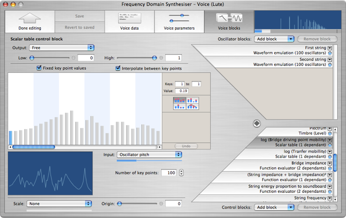
The bridge driving-point mobility directly affects how rapidly energy is transferred from the string to the soundboard, which in turn affects both the envelope decay rate and the level for each partial. Besides this, the soundboard resonances (here represented by a second table giving the bridge transfer mobility) affect the envelope attack rate and level for each partial.
To model both of these I have used a look-up table, whose input is the frequency of each oscillator, and whose output is used to modulate both the oscillator level and envelope times. Partials at frequencies where the mobility is high will lose energy quickly, giving a loud sound which decays quickly; where the mobility is low, the partials will be quieter but sustain for longer.
This example shows one of the unique features of the frequency domain architecture: the concept of "vector" control signals. These may be routed just like simple control signals, but instead of a single value, each vector signal carries a whole array of different values, one for each oscillator – 200 in this example. The input to the look-up table, "Oscillator pitch," is a vector control signal, and therefore so is its output. "Oscillator pitch" (which is an internal signal generated by the synthesiser itself) is a particularly important control signal because it is used to create all kinds of filters – a filter is just something which attenuates each partial by an amount which depends on the frequency of that partial.
I have given this voice a few performance parameters which allow the performer to control the plucking position and manner. These are shown off in the example sound clip, the Gavotte en Rondeau from the Partita in E major BWV1006a for keyboard or lute.
This voice leaves out a lot: it doesn't deal with the fact that the frequency response curve will be slightly different for each string, it ignores coupling between the strings, and although computationally cheap the look-up tables are not the most faithful way to model the resonances of the soundboard. On the whole, this voice is one part science and nine parts hand waving, and for some combinations of performance parameter values there is a noticeable electronic feel to the higher harmonics, but it still produces a reasonable first attempt.
Like the pipe model above, this voice shows how frequency domain synthesis blends features of other techniques. In this case, performance parameters affecting how a string is plucked can be handled well by a time-domain string model, but such models can only handle the soundboard's frequency response by recording or calculating a fixed sample of the soundboard's impulse response and playing it back through the waveguide filter representing the string. On the other hand, traditional additive synthesiser architectures can implement formant filters like the soundboard with ease, but would have more difficulty coping with the plucking parameters.